Genomics Workshop

Overview

In this 2-hour workshop, you will have hands-on experience on SNV calling and analysis. You will be provided toy short-read sequencing samples, followed by read alignments, variant calling and pathogenicity analysis.

Description

This workshop will guide you through the workflow of a simple genomic SNV analysis.

This is a hands-on workshop, which means you will be given time to get the tools running.

For each task, you will be given a brief instruction prior to getting your hands dirty. At the end of the given time, there will be a brief summary.

Pre-requisites

Basic knowledge of using command line and Rstudio is ideal. Although strictly speaking, no prior knowledge is required to attend this workshop.

Participation

The workshop runs for 2 hours. You will find tasks and related information in the worksheet.

If you run into any problems, please describe the issue and send via zoom chat. The instructors will be monitoring the chat panel and answer any question in real time.

Tools to be used

Time outline

For this 120-minute workshop:

Activity	Time
Introduction	5m
Working Environment: command line and Rstudio	15m
Read Alignment: bwa and samtools	20m
SNV calling: Strelka2	20m
Pathogenicity analysis	50m
Summary	10m

Workshop goals and objectives

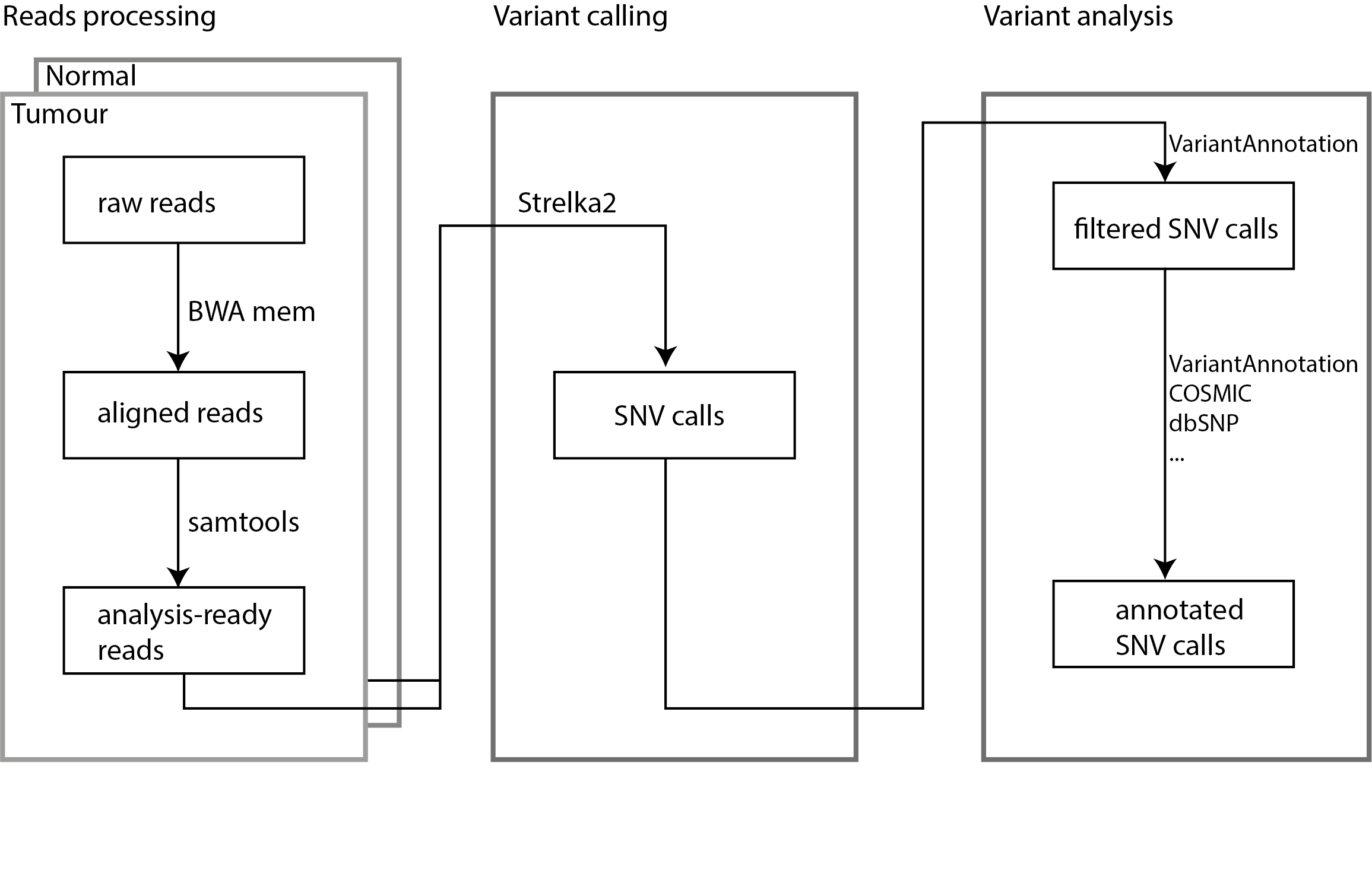
Variant calling is a vital component of genomics studies. Genomic variants have been found in various structures and sizes, including single-nucleotide variants (SNVs), small insertion and deletions (INDELs), copy number variants (CNVs) and structural variants (SVs). Computational tools for detecting these variants are developed with different underlying approaches.

This workshop is designed to offer a hands-on experience on genomic variant calling and analysis. The tasks are designed to guide you through the key steps of SNV analysis on a tumour/normal paired sample.

Learning goals

To understand the general workflow of a genomic variant analysis
To identify methods to handle short-read sequencing data and variant calls

Learning objectives

To recall the key concepts in genomic variant analysis
To apply the concepts in SNV calling to germline and paired tumour/normal data
To perform SNV analysis using publicly available resources

Workshop

Getting started

Rstudio working environment (console vs. terminal)
Data directory
Working with UNIX commands

working directories

cd colo829
ls

running cmd tools

samtools
man samtools #q for quitting the man page

piping

ls | head -3

SNV analysis workflow

Task 1: read alignments, sorting, and indexing

Here you will need to align short-read sequencing reads to the reference genome (hg19) and get them ready for SNV calling. There are two samples you will need the work with, the tumor sample and the matched normal sample of COLO829⁴.

Aligning reads to the reference genome

Typical human whole genome sequencing (WGS) data contains hundreds of millions or billions of reads. These data sets take many hours to align so for this workshop we are going to align a very small subset of real sequencing data.

The data we are using today is located in the colo829 directory. The reads can be found at /home/rstudio/colo829/*.fastq.gz, and the reference genome is located at /home/rstudio/colo829/chr7.fa.

Sequence alignment tools are command-line tools so for this first task, we are going to use the command-line terminal.

To start, let us navigate to the directory containing our data.

cd colo829
ls

The cd command is the “change directory” command. It changes our working directory from our “home” directory to the colo829 directory.

The ls command is the “list” command. It outputs all the files and directories in the current directory.

Our input data is paired-end sequencing data for a tumour sample and a matched normal.

This fastq files are output from the sequencing machine and we need to align them to the reference genome. In this workshop, we are going to use chromosome 7 of the hg19 human reference genome as our reference.

We will use bwa mem for our sequence alignment. If we type:

bwa mem

We see that bwa mem requires a reference genome, input file(s), and has many optional parameters. The reference genome is chr7.fa, and the files that start with chr7.fa..

Hint

bwa mem [options] <idxbase> <in1.fq> [in2.fq] > colo829.sam

Converting the output file format

The output file of bwa mem can be saved as a SAM file, standing for Sequence Alignment Map. For storage efficiency, SAM files are often losslessly compressed to BAM format, standing for Binary Alignment Map.

Try it yourself by modifying this template:

samtools view -S -b output.sam -o output.bam

This step is optional if you “pipe” your bwa output to samtools (see below).

Sorting and indexing

We also need to sort the output of bwa into the order in which they align in the reference genome. For this we will use samtools sort:

samtools sort

and samtools index:

samtools index

To avoid writing additional (uncompressed) files, we will combine the alignment and sorting steps together with a unix “pipe”. A pipe | takes the output from one program and sends it to the next program.

We can run our bwa and samtools commands together in a pipe using:

bwa mem chr7.fa normal_R1.fastq.gz normal_R2.fastq.gz | samtools sort - > normal.bam

Our variant caller requires a index file for our normal.bam file so we create this using samtools index:

samtools index normal.bam

As we are doing somatic variant calling, we need to repeat these steps on the tumour sequencing reads as well. Our tumour data is larger than our normal so to reduce the time it takes to perform alignment, we’ll tell bwa mem that it can use both CPU cores available to us in our workshop virtual machines by telling it to use 2 threads.

Now please try applying all the above steps on the tumour reads.

Solution

bwa mem -t 2 chr7.fa tumour_R1.fastq.gz tumour_R2.fastq.gz | samtools sort - > tumour.bam
samtools index tumour.bam

Task 2: calling SNVs using Strelka2

Now that we have the sequencing reads in order, we will start calling SNVs. We now have both the normal and tumour inputs ready for variant calling. In a real pipeline, there are additional quality control, adapter trimming, and duplicate filtering steps but for this workshop, the data has been pre-processed for us so we can skip these steps.

The variant caller we are using is Strelka2. Looking through the quick start guide, we can see that Strelka2 supports both somatic and germline variant calling. As we are doing somatic variant calling, we want to configure a somatic Strelka workflow

configureStrelkaSomaticWorkflow.py \
  --normalBam normal.bam \
  --tumorBam tumour.bam \
  --referenceFasta chr7.fa \
  --runDir strelka

This created a strelka subdirectory containing runWorkflow.py which is the command we will use to run Strelka.

strelka/runWorkflow.py

As we can see from the usage message, Strelka requires additional arguments. In our case, we want to specify that we will be running it on the same computer that we are running the runWorkflow.py command. We will also tell Strelka that it can use both the CPU cores available to us.

strelka/runWorkflow.py -j 2 -m local

If you navigate to the colo829/strelka/results/variants/ directory, you should now have a somatic.snvs.vcf.gz file containing the somatic variants that Strelka detected in our example sequencing data.

Task 3: investigating the driver gene

Load packages

library(VariantAnnotation)
library(TxDb.Hsapiens.UCSC.hg19.knownGene)
library(BSgenome.Hsapiens.UCSC.hg19)
library(org.Hs.eg.db)

Read and pre-process VCF file

We use the VariantAnnotation package to read and annotate the SNVs we just found.

#vcf <- readVcf(system.file("extdata", "strelka.somatic.vcf", package = #"IntroductionToGenomicsWorkshop"))
vcf <- readVcf("../inst/extdata/strelka.somatic.vcf")

Variant sequence style is changed to maintain its consistency with other databases.

seqlevelsStyle(vcf) <- "UCSC"

Header information of VCF file

header() function will show the header information from the VCF file.

header(vcf)
#> class: VCFHeader 
#> samples(2): NORMAL TUMOR
#> meta(12): cmdline content ... startTime contig
#> fixed(1): FILTER
#> info(22): AC AF ... TQSS_NT set
#> geno(15): AU CU ... TOR TU

Further information for the headers can be extracted by functions like samples(), geno(), meta(), etc.

Solution

This will fail.

samples(vcf)
#> Error in (function (classes, fdef, mtable) : unable to find an inherited method for function 'samples' for signature '"CollapsedVCF"'

These will work.

samples(header(vcf))
#> [1] "NORMAL" "TUMOR"
geno(vcf)
#> List of length 15
#> names(15): AU CU DP DP2 DP50 FDP FDP50 GU SDP SUBDP SUBDP50 TAR TIR TOR TU
head(geno(header(vcf)), 3)
#> DataFrame with 3 rows and 3 columns
#>         Number        Type            Description
#>    <character> <character>            <character>
#> AU           2     Integer Number of 'A' allele..
#> CU           2     Integer Number of 'C' allele..
#> DP           1     Integer   Read depth for tier1

Variant genomic position

The chromosomal location for each SNV can be identified by rowRanges().

head(rowRanges(vcf), 3)
#> GRanges object with 3 ranges and 5 metadata columns:
#>                seqnames    ranges strand | paramRangeID            REF
#>                   <Rle> <IRanges>  <Rle> |     <factor> <DNAStringSet>
#>    1:10250_A/C     chr1     10250      * |           NA              A
#>    1:10257_A/C     chr1     10257      * |           NA              A
#>   1:533197_A/G     chr1    533197      * |           NA              A
#>                               ALT      QUAL      FILTER
#>                <DNAStringSetList> <numeric> <character>
#>    1:10250_A/C                  C        NA        PASS
#>    1:10257_A/C                  C        NA        PASS
#>   1:533197_A/G                  G        NA        PASS
#>   -------
#>   seqinfo: 25 sequences from an unspecified genome

Individual fields can be pulled out either with the $ sign or named accessors like ref(), alt().

head(rowRanges(vcf)$ALT, 3)
#> DNAStringSetList of length 3
#> [[1]] C
#> [[2]] C
#> [[3]] G
head(alt(vcf), 3)
#> DNAStringSetList of length 3
#> [[1]] C
#> [[2]] C
#> [[3]] G

Locate variants in and around genes

Variant location with respect to genes can be identified with the locateVariants() function.

# Get variant location information.
rd <- rowRanges(vcf)
txdb <- TxDb.Hsapiens.UCSC.hg19.knownGene
loc <- locateVariants(rd, txdb, CodingVariants())
head(loc, 3)
#> GRanges object with 3 ranges and 9 metadata columns:
#>                seqnames    ranges strand | LOCATION  LOCSTART    LOCEND
#>                   <Rle> <IRanges>  <Rle> | <factor> <integer> <integer>
#>   1:883516_G/A     chr1    883516      - |   coding      1045      1045
#>   1:883516_G/A     chr1    883516      - |   coding      1654      1654
#>   1:883516_G/A     chr1    883516      - |   coding      1654      1654
#>                  QUERYID        TXID         CDSID      GENEID       PRECEDEID
#>                <integer> <character> <IntegerList> <character> <CharacterList>
#>   1:883516_G/A        18        4114         12095       26155                
#>   1:883516_G/A        18        4115         12095       26155                
#>   1:883516_G/A        18        4116         12095       26155                
#>                       FOLLOWID
#>                <CharacterList>
#>   1:883516_G/A                
#>   1:883516_G/A                
#>   1:883516_G/A                
#>   -------
#>   seqinfo: 25 sequences from an unspecified genome; no seqlengths

Gene ID can be replaced my gene symbols which are more readable, using org.HS.eg.db database.

gene_symbol <- biomaRt::select(org.Hs.eg.db, keys=loc$GENEID, columns=c("SYMBOL"), keytype="ENTREZID")$SYMBOL
head(gene_symbol, 5)
#> [1] "NOC2L"  "NOC2L"  "NOC2L"  "PRDM16" "PRDM16"
loc$SYMBOl <- gene_symbol
head(loc, 3)
#> GRanges object with 3 ranges and 10 metadata columns:
#>                seqnames    ranges strand | LOCATION  LOCSTART    LOCEND
#>                   <Rle> <IRanges>  <Rle> | <factor> <integer> <integer>
#>   1:883516_G/A     chr1    883516      - |   coding      1045      1045
#>   1:883516_G/A     chr1    883516      - |   coding      1654      1654
#>   1:883516_G/A     chr1    883516      - |   coding      1654      1654
#>                  QUERYID        TXID         CDSID      GENEID       PRECEDEID
#>                <integer> <character> <IntegerList> <character> <CharacterList>
#>   1:883516_G/A        18        4114         12095       26155                
#>   1:883516_G/A        18        4115         12095       26155                
#>   1:883516_G/A        18        4116         12095       26155                
#>                       FOLLOWID      SYMBOl
#>                <CharacterList> <character>
#>   1:883516_G/A                       NOC2L
#>   1:883516_G/A                       NOC2L
#>   1:883516_G/A                       NOC2L
#>   -------
#>   seqinfo: 25 sequences from an unspecified genome; no seqlengths

The number of SNVs on each chromosome can be displayed by seqnames().

seqnames(loc)
#> factor-Rle of length 918 with 23 runs
#>   Lengths:    94    99    53    55    31 ...    66    12    10    14    27
#>   Values : chr1  chr2  chr3  chr4  chr5  ... chr19 chr20 chr21 chr22 chrX 
#> Levels(25): chr1 chr2 chr3 chr4 chr5 chr6 ... chr20 chr21 chr22 chrX chrY chrM

The documentation of locateVariants() describes how to identify variants in other regions, like splicing sites.

Solution

Check the documentation of locateVariants().

?locateVariants

Following functions are used to identify variants in distinct gene regions:

Function	Description
CodingVariants()	Falls within a coding region
IntronVariants()	Falls within an intron region
FiveUTRVariants()	Falls within a 5’ untranslated region
ThreeUTRVariants()	Falls within a 3’ untranslated region
IntergenicVariants()	Does not fall within a transcript associated with a gene
SpliceSiteVariants()	Overlaps any portion of the first 2 or last 2 nucleotide of an intron
PromoterVariants()	Falls within a promoter region of a transcript
AllVariants()	All regions

loc_splice <- locateVariants(rd, txdb, SpliceSiteVariants())
head(loc_splice, 3)
#> GRanges object with 3 ranges and 9 metadata columns:
#>                seqnames    ranges strand |   LOCATION  LOCSTART    LOCEND
#>                   <Rle> <IRanges>  <Rle> |   <factor> <integer> <integer>
#>   1:787492_T/C     chr1    787492      + | spliceSite      <NA>      <NA>
#>   1:787492_T/C     chr1    787492      + | spliceSite      <NA>      <NA>
#>   1:787492_T/C     chr1    787492      + | spliceSite      <NA>      <NA>
#>                  QUERYID      TXID         CDSID      GENEID       PRECEDEID
#>                <integer> <integer> <IntegerList> <character> <CharacterList>
#>   1:787492_T/C        12        15                    643837                
#>   1:787492_T/C        12        16                    643837                
#>   1:787492_T/C        12        18                    643837                
#>                       FOLLOWID
#>                <CharacterList>
#>   1:787492_T/C                
#>   1:787492_T/C                
#>   1:787492_T/C                
#>   -------
#>   seqinfo: 25 sequences from an unspecified genome; no seqlengths
seqnames(loc_splice)
#> factor-Rle of length 38 with 7 runs
#>   Lengths:     6     7    13     1     4     1     6
#>   Values : chr1  chr2  chr3  chr4  chr9  chr11 chr16
#> Levels(25): chr1 chr2 chr3 chr4 chr5 chr6 ... chr20 chr21 chr22 chrX chrY chrM

Amino acid coding changes

predictCoding computes amino acid coding changes for non-synonymous mutations.

coding <- predictCoding(vcf, txdb, seqSource = Hsapiens)
coding[3:4]
#> GRanges object with 2 ranges and 17 metadata columns:
#>                 seqnames    ranges strand | paramRangeID            REF
#>                    <Rle> <IRanges>  <Rle> |     <factor> <DNAStringSet>
#>    1:883516_G/A     chr1    883516      - |           NA              G
#>   1:3329312_C/T     chr1   3329312      + |           NA              C
#>                                ALT      QUAL      FILTER      varAllele
#>                 <DNAStringSetList> <numeric> <character> <DNAStringSet>
#>    1:883516_G/A                  A        NA        PASS              T
#>   1:3329312_C/T                  T        NA        PASS              T
#>                    CDSLOC    PROTEINLOC   QUERYID        TXID         CDSID
#>                 <IRanges> <IntegerList> <integer> <character> <IntegerList>
#>    1:883516_G/A      1654           552        18        4116         12095
#>   1:3329312_C/T      2551           851        79         154           395
#>                      GENEID   CONSEQUENCE       REFCODON       VARCODON
#>                 <character>      <factor> <DNAStringSet> <DNAStringSet>
#>    1:883516_G/A       26155 synonymous               CTG            TTG
#>   1:3329312_C/T       63976 nonsynonymous            CCC            TCC
#>                         REFAA         VARAA
#>                 <AAStringSet> <AAStringSet>
#>    1:883516_G/A             L             L
#>   1:3329312_C/T             P             S
#>   -------
#>   seqinfo: 25 sequences from an unspecified genome

Here shows all consequences of coding variants.

table(coding$CONSEQUENCE)
#> 
#>    frameshift      nonsense nonsynonymous    synonymous 
#>            21            46           562           289

We can also annotate each of these variants with their corresponding gene by looking up the GENEID.

coding$SYMBOL <- biomaRt::select(org.Hs.eg.db, keys=coding$GENEID, columns=c("SYMBOL"), keytype="ENTREZID")$SYMBOL
#> 'select()' returned many:1 mapping between keys and columns
coding[3:4]
#> GRanges object with 2 ranges and 18 metadata columns:
#>                 seqnames    ranges strand | paramRangeID            REF
#>                    <Rle> <IRanges>  <Rle> |     <factor> <DNAStringSet>
#>    1:883516_G/A     chr1    883516      - |           NA              G
#>   1:3329312_C/T     chr1   3329312      + |           NA              C
#>                                ALT      QUAL      FILTER      varAllele
#>                 <DNAStringSetList> <numeric> <character> <DNAStringSet>
#>    1:883516_G/A                  A        NA        PASS              T
#>   1:3329312_C/T                  T        NA        PASS              T
#>                    CDSLOC    PROTEINLOC   QUERYID        TXID         CDSID
#>                 <IRanges> <IntegerList> <integer> <character> <IntegerList>
#>    1:883516_G/A      1654           552        18        4116         12095
#>   1:3329312_C/T      2551           851        79         154           395
#>                      GENEID   CONSEQUENCE       REFCODON       VARCODON
#>                 <character>      <factor> <DNAStringSet> <DNAStringSet>
#>    1:883516_G/A       26155 synonymous               CTG            TTG
#>   1:3329312_C/T       63976 nonsynonymous            CCC            TCC
#>                         REFAA         VARAA      SYMBOL
#>                 <AAStringSet> <AAStringSet> <character>
#>    1:883516_G/A             L             L       NOC2L
#>   1:3329312_C/T             P             S      PRDM16
#>   -------
#>   seqinfo: 25 sequences from an unspecified genome

We can discard the synonymous mutations, and the rest are potential cancer drivers. Then map them back to the VCF data and filter it.

potential_drivers = coding[!is.na(coding$CONSEQUENCE) & coding$CONSEQUENCE != "synonymous"]
potential_drivers = rowRanges(vcf)[overlapsAny(rowRanges(vcf), potential_drivers, ignore.strand=TRUE)]

Predict impact

For the nonsynonymous mutations, we’d like to know how much these impact the protein. For this, we will use to pre-calculated scores from the rfPred package. To work out how to use the package, we look up the help.

`?rfPred-package`

If you click on the index link, it will show you all functions available in the package. Check what the scoring function requires we see the variant_list parameter requires a data.frame with specific columns. We’ll need to create that before calling the function.

library(rfPred)
rfpred_gr = potential_drivers
seqlevelsStyle(rfpred_gr) = "NCBI"
rfpred_df = data.frame(
  seqnames=seqnames(rfpred_gr),
  start=start(rfpred_gr),
  reference=as.character(rfpred_gr$REF),
  alteration =as.character(unlist(rfpred_gr$ALT)))
scores = rfPred::rfPred_scores(
  variant_list=rfpred_df, 
  data="/home/rstudio/rfPred/all_chr_rfPred.txtz",
  index="/home/rstudio/rfPred/all_chr_rfPred.txtz.tbi")
scores = scores[order(-as.numeric(scores$rfPred_score)),]
head(scores, 20)

Match variants within COSMIC

To work out which variants are likely driver genes, we can check if they have been seen before in COSMIC

Read and pre-process COSMIC database.

cosmic_path <- system.file("vcf", "cosmic_67.vcf.gz", package = "COSMIC.67")
cosmic_db <- readVcf(cosmic_path, genome = "GRCh37")
seqlevelsStyle(cosmic_db) <- "UCSC"

The potential driver variants are matched with the COSMIC database.

# Match by chromosome and location of the variants.
cosmics_hits = findOverlaps(potential_drivers, rowRanges(cosmic_db), type="equal")
#> Warning in .Seqinfo.mergexy(x, y): Each of the 2 combined objects has sequence levels not in the other:
#>   - in 'x': chrM
#>   - in 'y': chrMT
#>   Make sure to always combine/compare objects based on the same reference
#>   genome (use suppressWarnings() to suppress this warning).
# Match by reference and alternative allele of the variants.
cosmics_hits = cosmics_hits[
  as.character(potential_drivers$REF[queryHits(cosmics_hits)]) == as.character(rowRanges(cosmic_db)$REF[subjectHits(cosmics_hits)]) &
  as.character(unlist(potential_drivers$ALT[queryHits(cosmics_hits)])) == as.character(unlist(rowRanges(cosmic_db)$ALT[subjectHits(cosmics_hits)]))
  ]

Finally, we take the COSMIC information of the potential driver mutants and rank them by CNT. CNT values denote the sample count for the given variant.

found_in_cosmic = info(cosmic_db)[subjectHits(cosmics_hits),]
found_in_cosmic = found_in_cosmic[order(-found_in_cosmic$CNT),]
found_in_cosmic = found_in_cosmic[!is.na(found_in_cosmic$CNT),]
head(found_in_cosmic, 5)
#> DataFrame with 5 rows and 5 columns
#>                              GENE      STRAND         CDS          AA       CNT
#>                       <character> <character> <character> <character> <integer>
#> COSM476                      BRAF           -   c.1799T>A     p.V600E     19691
#> COSM25632                   AGFG1           +   c.1018G>A     p.G340R         7
#> COSM1405984 AGFG1_ENST00000409979           +   c.1090G>A     p.G364R         5
#> COSM226579  STK19_ENST00000375333           +    c.265G>A      p.D89N         5
#> COSM23305                   HDAC2           -   c.1225C>T     p.R409*         4

Now you can search the mutation identifier (COSM476 for example) in COSMIC and learn more about the variant.

dong.rn@wehi.edu.au ↩︎
fu.j@wehi.edu.au ↩︎
cameron.d@wehi.edu.au ↩︎
Craig, D., Nasser, S., Corbett, R. et al. A somatic reference standard for cancer genome sequencing. Sci Rep 6, 24607 (2016). https://doi.org/10.1038/srep24607 ↩︎

Ruining Dong¹

James Fu²

Daniel Cameron³

Overview

Description

Pre-requisites

Participation

Tools to be used

Time outline

Workshop goals and objectives

Learning goals

Learning objectives

Workshop

Getting started

Task 1: read alignments, sorting, and indexing

Aligning reads to the reference genome

Converting the output file format

Sorting and indexing

Task 2: calling SNVs using Strelka2

Task 3: investigating the driver gene

Load packages

Read and pre-process VCF file

Header information of VCF file

Variant genomic position

Locate variants in and around genes

Amino acid coding changes

Predict impact

Match variants within COSMIC

Genomics Workshop

Ruining Dong1

James Fu2

Daniel Cameron3

Overview

Description

Pre-requisites

Participation

Tools to be used

Time outline

Workshop goals and objectives

Learning goals

Learning objectives

Workshop

Getting started

Task 1: read alignments, sorting, and indexing

Aligning reads to the reference genome

Converting the output file format

Sorting and indexing

Task 2: calling SNVs using Strelka2

Task 3: investigating the driver gene

Load packages

Read and pre-process VCF file

Header information of VCF file

Variant genomic position

Locate variants in and around genes

Amino acid coding changes

Predict impact

Match variants within COSMIC

Ruining Dong¹

James Fu²

Daniel Cameron³